Fundamentals of Linear Regression

In this post, we investigate one of the most common and widely used machine learning techniques: linear regression.

Linear regression is a very intuitive supervised learning algorithm and as its name suggests, it is a regression technique. This means it is used when we have labels that are continuous values such as car prices or the temperature in a room. Furthermore, as its name also suggests, linear regression seeks to find fits of data that are lines. What does this mean?

Motivations

Imagine that you received a data set consisting of cars, where for each car you had the number of miles a car had driven along with its price. In this case, let’s assume that you are trying to train a machine learning system that takes in the information about each car, namely the number of miles driven along with its associated price.

Here for a given car, the miles driven is the input and the price is the output. This data could be represented as $(X, Y)$ coordinates.

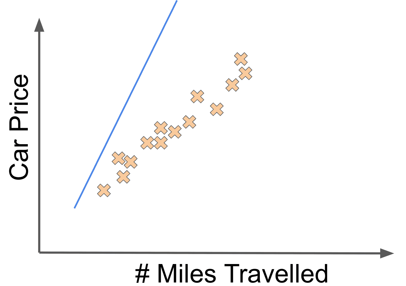
Plotting them on a 2-d coordinate system, this data could might look like:

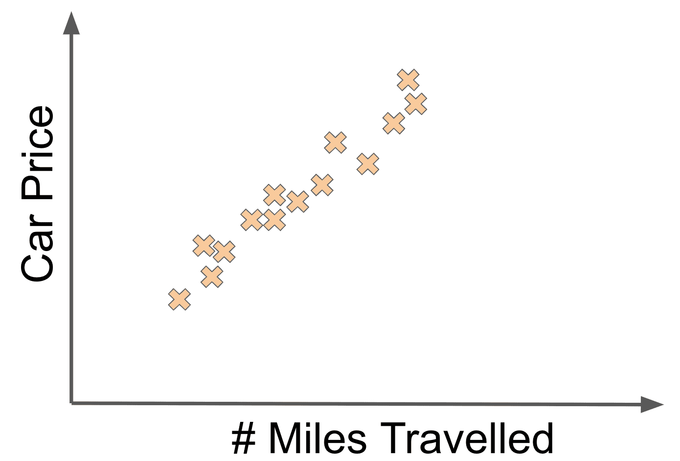
In this case, it seems that there is a linear relationship between the miles driven and the price. If we fit a reasonable looking line to the data, it could look like:

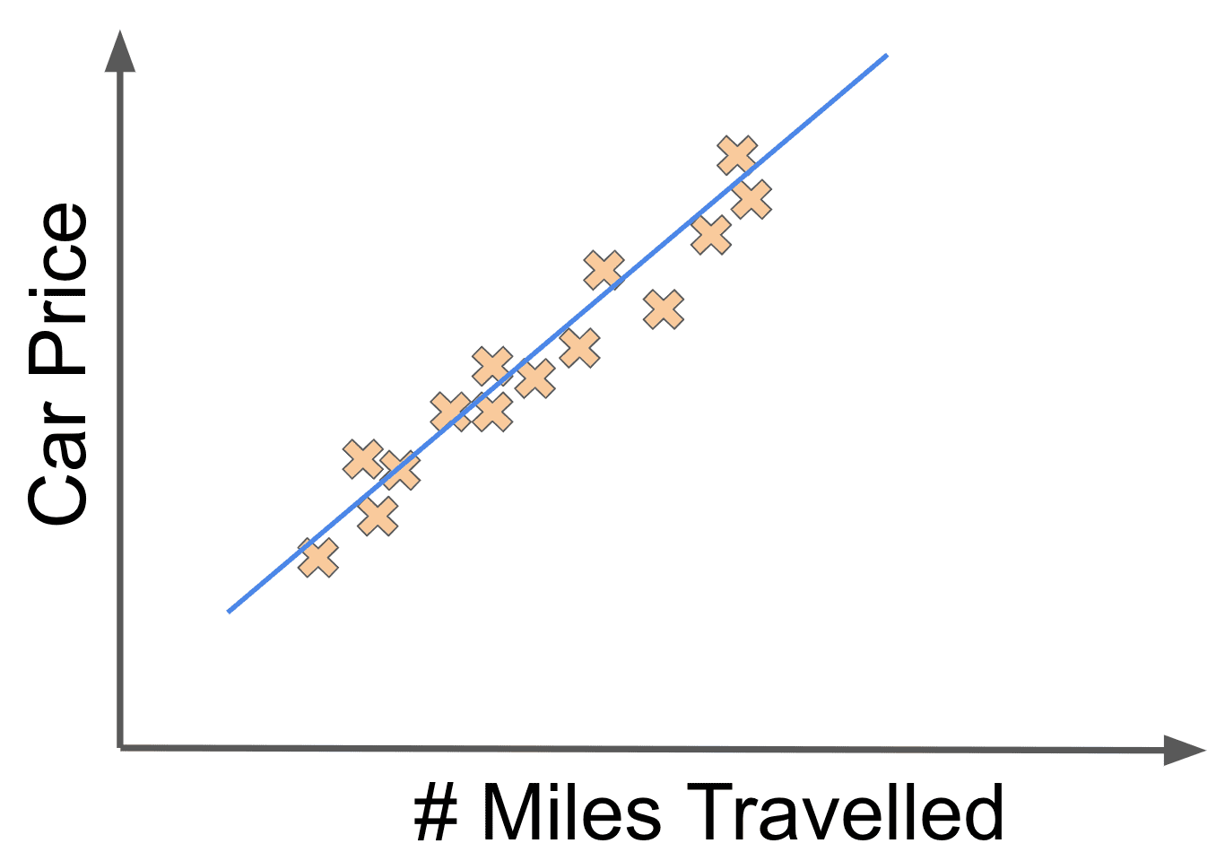
We could describe the model for our car price dataset as a mathematical function of the form: $F(X) = A_1 \cdot X + A_0$

Here $A_1$ and $A_0$ are called weights and these are the values that determine how our linear function behaves on different inputs. All supervised learning algorithms have some set of weights that determine how the algorithm behaves on different inputs, and determining the right weights is really at the core of what we call learning.

Let’s say that the linear fit above was associated with the weights $A_1 = 5$ and $A_0 = 0.5$. Now if we changed the $A_0$ value to something like $A_0 = -2$, we might get the following linear fit:

Or imagine that we thought that there was a much steeper relationship between the number of miles driven and a car’s price. In other words, we think the $A_1$ value (which here determines the slope of the line) should be a bigger value such as 8. Our linear fit would then look like this:

A Training Paradigm

These varieties of linear fits raise the question: how do we actually learn the weights of this model or any machine learning model in general? In particular, how can we leverage the fact that we have the correct labels for the cars in our dataset?

Training and evaluating a machine learning model involves using something called a cost function. In the case of supervised learning, a cost function is a measure of how much the predicted labels outputted by our model deviate from the true labels. Ideally we would like the deviation between the two to be small, and so we want to minimize the value of our cost function.

A common cost function used for evaluating linear regression models is called the least-squares cost function. Let’s say that we have $n$ datapoints in our data set.

This could look like $[(X_1, Y_1), (X_2, Y_2), ... , (X_n, Y_n)]$.

If we are learning a function $F(X)$, the least-squares regression model seeks to minimize:

The deviation between our predicted output ($F(X)$) and the true output ( $Y$) is defined as a residual. The least-squares cost is trying to minimize the sum of the squares of the residuals (multiplied by a constant in this case).

Here it is important to note that $F(X)$ is a function of the weights of our model. In our motivating example, $F(X)$ would be a function of $A_1$ and $A_0$. The values of $A_1$ and $A_0$ that produce our optimal model are the values which achieve the minimal value of $C(X)$.

How do we actually compute the weights that achieve the minimal values of our cost? Here, as with all machine learning models, we have two options: an analytical or a numerical solution. In an analytical solution, we seek to find an exact closed-form expression for the optimal value. In this particular case, that involves using standard calculus optimization. We would take the gradients (which are just fancy derivatives) of the cost function with respect to the weights, set those gradients to 0, and then solve for the weights that achieve the 0 gradient.

This technique is nice because once we have computed the closed-form expression for the gradients, we can get the optimal weight values for any new data. Here we are able to develop an analytical solution in the case of linear regression with a least-squares cost function.

However, not all models have nice well-formed gradient expressions that allow us to solve for the global optimum of a problem. For these problems, we must turn to numerical methods. Numerical methods typically involve a step-wise update procedure that iteratively brings weights closer to their optimal value. Here we again compute the gradients with respect to all the weights and then apply the following update for each weight $A$:

We continue applying these updates for some number of iterations until our weight values converge, by which I mean to say they don’t change too much from one iteration to the next. This very important numerical optimization procedure is called gradient descent.

Note in our expression for gradient descent above, we have this magical alpha ($\alpha$) value being multiplied to the gradient. Alpha is an example of what is called in machine learning a hyperparameter. The value of this hyperparameter alpha determines how quickly updates are made to our weights. We are free to adjust the value so that gradient descent converges more quickly.

Many machine learning algorithms have their own hyperparameters that we can adjust and fine-tune to achieve better performance in our algorithm. For some algorithms, such as in deep learning, hyperparameter tuning is a super important task that can drastically impact how good of a system we build.

In the case of linear regression with a least-squares cost we are guaranteed that gradient descent will eventually converge to the optimal weight values. However, certain optimization problems don’t have that guarantee, and the best we can hope for is that gradient descent converges to something close to the global optimum. A prominent example of models with this behavior are deep learning models, which we will discuss in greater depth later.

An important point to keep in mind is that in the original linear model we proposed we only have two weights, $A_1$ and $A_0$. But what if we really believed that car prices were a function of two features, the number of miles driven and the size of the trunk space in cubic feet?

Now if we wanted to train a linear regression model, our dataset would have to include the number of miles driven, the size of the trunk space, and the price for every car. We would also now have three weights in our linear regression model: $A_0$, $A_1$, and $A_2$.

Furthermore, our data would now exist in a 3-d coordinate system, not a 2-d one. However, we could use the same least-squares cost function to optimize our model. As we increase the number of features, the same basic algorithmic considerations apply with a few caveats. We will discuss these caveats when we discuss the bias-variance tradeoff.

When Does a Linear Fit Fit?

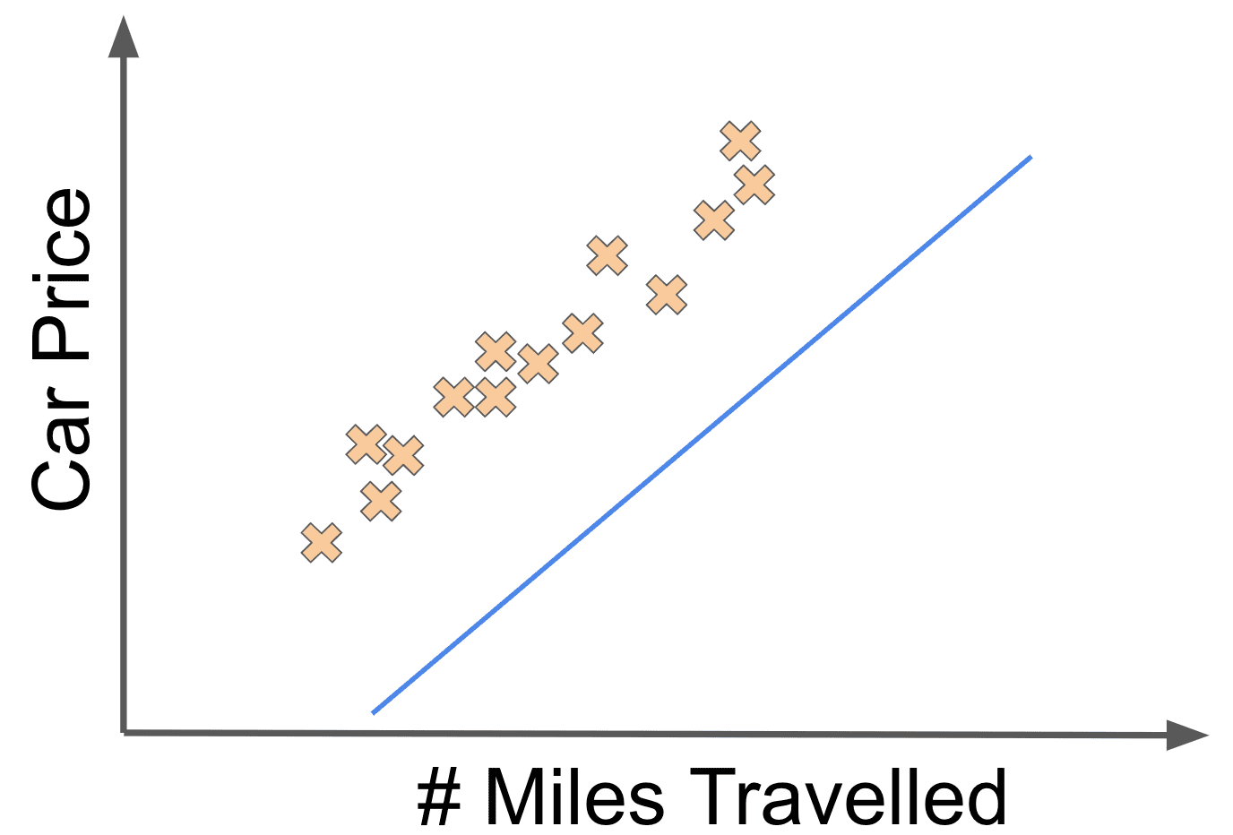
When does linear regression work well as a modelling algorithm choice? In practice, it turns out that linear regression works best when there actually is a linear relationship between the inputs and the outputs of your data. For example, if our car price data looked as follows:

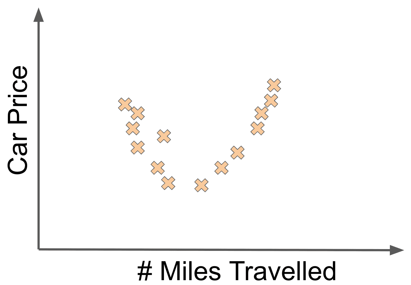
then linear regression probably would not be a good modelling choice.

When we are building a machine learning system, there are a few factors that we have to determine. First off, we need to extract the correct features from our data. This step is crucial!

In fact, this step is so important that for decades the contributions of many artificial intelligence papers were just different set of features to use for a particular problem domain. This style of paper has become not as prevalent with the resurgence of deep learning 🙂.

After selecting features, we need to pick the right modelling algorithm to fit. For example, if we think there is a linear relationship between our inputs and outputs, a linear regression may make sense. However, if we don’t think a line makes sense, we would pick a different model that has some different assumptions about the underlying structure of the data. We will investigate many other classes of models with their assumptions about the data in later posts.

Shameless Pitch Alert: If you’re interested in practicing MLOps, data science, and data engineering concepts, check out Confetti AI the premier educational machine learning platform used by students at Harvard, Stanford, Berkeley, and more!